
Table of Contents

Optimizing OpenSearch performance by profiling queries and shifting costly operations to write-time, improving throughput, and reducing latency.
Handling fluctuating workloads is a difficult task in many databases, as adding more resources is both costly and time consuming, and avoiding downtime is vital. This post will outline our methodology for identifying where we should focus our efforts in improving performance, and what techniques we’ve used to greatly improve our overall query throughput.
We’ll go over identifying the areas in need of improvement, profiling queries to understand what makes them take long, and ways we’ve utilized this data to improve performance of these queries.
Motivation
Unlike many other processes, scaling an OpenSearch cluster takes at least several hours, making it impractical to scale up or down in response to temporary traffic spikes. It’s a bit like city traffic: you can’t just build more roads every time there’s a jam.
This means that before committing to increasing our cluster size, we first wanted to make sure we’re not wasting resources – maybe we can reach higher max throughput with the same hardware, just used more efficiently.
The Symptoms
So how do we determine there actually is an issue with performance? In our case, it was pretty straightforward – OpenSearch could not handle all the queries being sent and started responding with 429 `Too many requests` errors. Looking at the diagnostic data, we saw that during the times of unavailability, the cluster reached 100% CPU usage, and queries took so long that they clogged the thread queue.
Finding the Costly Queries
While at first we tried using the built-in tools for identifying slow queries, we quickly found that the slow queries weren’t any different from the quick ones – they just had the misfortune of being sent while the cluster was struggling. So instead of looking for individually problematic queries, we were looking for common queries that were costly in terms of compute resources. Optimizing an inefficient query pattern that runs rarely won’t meaningfully reduce overall cluster load.
Fortunately, identifying frequent queries was straightforward: we analyzed our logs to find the most common query patterns.
One pattern in particular stood out as both frequent and potentially inefficient, making it a strong candidate for optimization:
{
  "query": {
    "bool": {
      "filter": [
        {
          "bool": {
            "must_not": [
              { "term": { "categorical_a": "value_a" } },
              { "term": { "categorical_a": "value_b" } }
            ]
          }
        }
      ],
      "should": [
        {
          "multi_match": {
            "query": "sample query",
            "fields": ["text_a", "text_b"]
          }
        },
        {
          "bool": {
            "must": [
              { "rank_feature": { "field": "scalar_a", "boost": 3 } },
              { "rank_feature": { "field": "scalar_b", "boost": 2 } }
            ]
          }
        }
      ],
      "minimum_should_match": 2
    }
  }
}This (slightly simplified) sample query is made of three main parts:
- a must_not filter, which filters out records with specific categorical fields
- a multi_match, which utilizes OpenSearch’s full-text search
- two rank_feature scalars, which boost results to earlier results based on numerical fields
Profiling
With a sample query in hand, we used a sample query with the `profile` flag to analyze how much time each part of the query consumes.
While reducing query latency is a nice side effect, our primary goal was to lower CPU usage and prevent them from clogging the cluster’s processing queues.
Let’s look at the result of the profiled query:
{
  "query": [
    {
      "type": "BooleanQuery",
      "time": "24.8ms",
      "children": [
        {
          "type": "BoostQuery",
          "description": "(((text_a:sample query) | (text_b:sample query)))",
          "time": "5.1ms"
        },
        {
          "type": "BooleanQuery",
          "description": "+(FeatureQuery(field=_feature, feature=scalar_a)))^3.0 +(FeatureQuery(field=_feature, feature=scalar_b))^2.0",
          "time": "11.3ms"
        },
        {
          "type": "BooleanQuery",
          "description": "-categorical_a:value_a -categorical_a:value_b #*:*",
          "time": "5.2ms"
        }
      ]
    }
  ]
}The actual profile result is much longer, and includes the time it took in each shard as well as other useful information, but for our purposes this simplified example is clearer
Examining the `profile` section of the response revealed a surprising result:
Most of the time was spent on categorical filtering and boosting.
This wasn’t what we expected, but it’s actually encouraging. If we can avoid those parts of the query, we should be able to significantly reduce resource consumption – and improve performance along the way.
Avoiding Filters
By default, all queries of the targeted pattern included two categorical filters, which together excluded about 20% of our data. Rather than repeatedly filtering out the same records at query time, we realized we could simply… not store them in the first place.
By duplicating the data into a secondary index containing only the relevant records, we could bypass those filters entirely, without impacting other query types that don’t rely on this filtering logic.
When we originally added the filters, we didn’t anticipate such a significant performance impact. This is exactly where profiling proves its value.
Pre-Computing Features
Another unexpected insight from profiling was the cost of using two rank_feature fields for boosting. Although the features themselves were static, OpenSearch had to compute their combined effect at query time. Much like the filters, this computation could be offloaded to index-time instead of being done during each query
To achieve this, we needed to replicate the logic OpenSearch uses when combining multiple rank_features fields. The exact computation depends on how your index is configured – whether you’re using the saturation, log, or sigmoid function.
By default, OpenSearch applies the saturation function with a dynamically computed pivot value, then sums the results of all rank_features fields (applying individual boosts if specified).
Most of this is straightforward to precompute at write-time. However, if you haven’t explicitly set a pivot, OpenSearch derives it at query time. According to the documentation, the default pivot is an approximation of the geometric mean of all values for that field. You can also inspect the actual pivot used by examining the `profile` query, and inspect the actual pivot value used to verify this.
It’s worth noting that the pivot value can drift slightly as new documents are added. In our case, this wasn’t an issue as we wrote the entire index in a single batch and never updated it. Whenever we need fresh data, we create a new index from scratch. However, if your workflow involves frequent updates to the index, you should test whether pivot drift affects your use case. It might be negligible (especially if one rank_feature dominates the final result), but it’s something to be aware of.
Segment Merging
It’s the oldest trick in the book, but as long as it works, it deserves to stay there. Reducing the number of segments can have a dramatic impact on query performance. Our initial goal was to target segment sizes just under 5 GB, but even conservative force merges that left most segments at 100s of MB helped a lot.
Keep in mind that force merges are irreversible (unless you rewrite the index), so when experimenting to find the optimal segment size, it’s convenient to begin with a higher segment count and gradually reduce it over multiple trials.
An alternative approach (less documented but very effective) is to skip force merges entirely and instead adjust the `merge.policy.floor_segment` setting to a higher value than the default 2 MB. We settled on 500 MB. This allows OpenSearch’s background merge process to consolidate segments more aggressively without requiring precise tuning.
There’s no one-size-fits-all answer for the ideal number of segments. The right configuration depends on your data and your cluster. Experimenting here can go a long way.
Operational Cost
Optimization doesn’t come for free. Even setting aside the time spent diagnosing the problem and experimenting with solutions, our new indexing approach introduces real overhead.
We now have to precompute compound boost values, write two separate (though similar) indices, and keep them in sync. This added complexity carries an operational cost.
That said, the trade-off has been well worth it: it enabled us to use our cluster far more efficiently during query execution.
Results
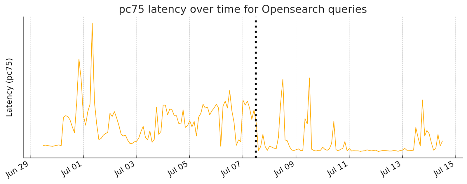
Our main goal was to increase the max throughput before we start experiencing unavailability. It’s difficult to measure how many issues would happen if we hadn’t optimized the index, so we’ll have to use imperfect proxies instead. One such proxy is the latency of queries over time. We can see in the graph below that before we deployed the update, query performance started to degrade even at moderate usage, and got really bad at peak usage times. After the update, there’s still some degradation at the peak times, but not as bad and for much more limited amounts of time. Most of the time at low to moderate usage, the latency is much lower
Looking at the profile results, the same query as before (after being adapted to use the new index) looks much better:
{
  "query": [
    {
      "type": "BooleanQuery",
      "time": "5.8ms",
      "children": [
        {
          "type": "BoostQuery",
          "description": "(((text_a:sample query) | (text_b:sample query)))",
          "time": "2.3ms"
        },
        {
          "type": "FeatureQuery",
          "description": "FeatureQuery(field=_feature, feature=compound_scalar)",
          "time": "2.5ms"
        }
      ]
    }
  ]
}The query takes much less time, and boosting a single rank_feature with a linear function takes much less than two features with runtime-derived values.
Summary
We started with a simple goal: handle peak loads more efficiently without scaling our OpenSearch cluster.
Along the way, profiling helped uncover unexpected bottlenecks like categorical filters and boosting logic, that we could shift from query-time to write-time. With a few targeted changes, including precomputing features, splitting indices, and reducing segment count, we significantly improved query performance and enabled our original goal of increasing the overall throughput of the cluster.