Feature Engineering for B2B Lead Scoring: Which External Signals Actually Move the Needle

TL;DR

• Internal CRM data alone underfits B2B lead scoring models because it captures only a fraction of the signals that predict purchase intent.
• External signals span five major categories: firmographic, technographic, intent, behavioral, and news or event-driven signals.
• Waterfall enrichment dramatically reduces feature sparsity by cascading across 50+ data sources until a field is populated.
• Model drift in B2B scoring is often driven by macro shifts in external signal distributions, not just label drift.
• SHAP values and permutation importance reveal which external features contribute most lift, guiding future data investment.
• Explorium’s AgentSource MCP server delivers enriched feature vectors at 100 QPS, making real-time scoring pipelines practical.
• Practical Python pipelines can transform raw external signals into model-ready features with proper imputation and encoding.

Most B2B lead scoring models plateau. They start strong, powered by CRM fields like industry, employee count, and deal history, and then stagnate. Precision hovers at 0.55. AUC sits at 0.71. The model keeps promoting accounts that never convert and buries accounts that close in days. If that sounds familiar, the root cause is almost always the same: you are asking a model to predict complex purchase behavior using features that describe only the buyer’s administrative profile, not their actual readiness to buy.

The solution is not a better algorithm. It is better features. Specifically, it is the category of features that internal data can never provide: external signals that reflect what a company is doing right now, what technologies they run, what topics their team is researching, and what events are reshaping their priorities. Feature engineering for B2B lead scoring is fundamentally a data problem before it is a modeling problem, and this article is a detailed practitioner’s guide to solving it.

We will cover the full taxonomy of external signals, how to build pipelines that handle sparse and missing data at enterprise scale, how to detect and respond to model drift, and how to measure feature importance in a way that actually informs your next enrichment investment. Every section includes real code and real metrics so you can move from concept to implementation.

Why CRM Features Alone Underfit B2B Lead Scoring Models

CRM data is retrospective by design. It captures what happened after a human decided to log it. Firmographic fields like company size, industry vertical, and revenue band are static attributes that describe the structural profile of an account, not its current state of mind. They tell you whether a company could buy, not whether it is about to. The result is a model trained almost entirely on demographic proxies, and demographic proxies have a fundamental ceiling on predictive power for conversion outcomes.

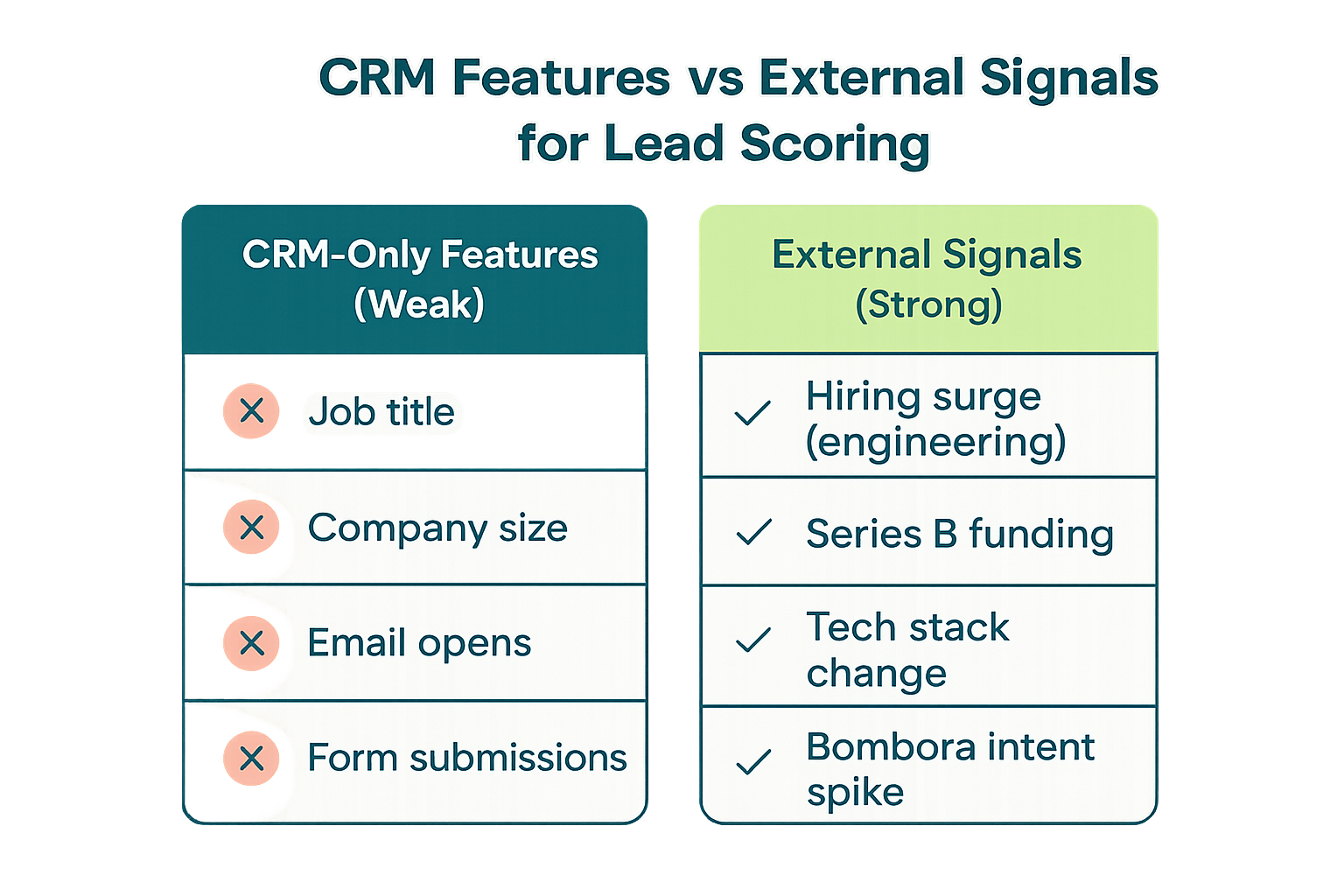
To understand why, consider the information asymmetry in a typical B2B dataset. When a deal closes, you might have 15 to 20 CRM fields populated for that account. But the buying decision was influenced by hundreds of signals that were never captured: a competitor’s contract expiring, a new CISO who ran a competing stack at their last company, a spike in job postings for roles that need the exact capability your product provides, a surge in research activity on Bombora-tracked topics matching your category. None of that is in your CRM. All of it is predictive.

Empirically, the underfitting shows up in several places. First, your model’s lift curve is flat beyond the top decile. If you sort your scored leads by predicted probability and only the top 10% show meaningful conversion lift, your model has essentially learned a simple rule and cannot generalize it. Second, feature importance analysis reveals that two or three demographic fields dominate, while everything else contributes negligible signal. Third, your model degrades quickly over time even when you retrain on fresh labels, because the features themselves are not tracking the dynamic world the buyer operates in.

The fix requires expanding the feature space beyond what any single internal system can provide. Research from multiple enterprise ML teams consistently shows that adding external enrichment data to B2B scoring models improves AUC by 8 to 15 percentage points on average. The catch is that external data introduces new engineering challenges: missing values, schema inconsistencies across providers, temporal staleness, and distribution shifts that cause model drift. Solving those challenges is what this guide is about.

The table above reflects benchmarks from teams that have gone through this journey. The numbers are not hypothetical. They reflect what happens when you give a gradient boosting model real behavioral context instead of asking it to infer intent from demographic proxies. The jump from 0.72 to 0.85 AUC is the difference between a model your sales team ignores and one that drives prioritization decisions every morning.

The Taxonomy of External Signals for B2B Lead Scoring

Not all external signals are equal, and conflating them is one of the most common mistakes in feature engineering for B2B lead scoring. Different signal types have different update frequencies, different coverage rates, different predictive windows, and different engineering requirements. Understanding the taxonomy lets you allocate your data budget intelligently and design pipelines that handle each signal type appropriately.

Firmographic Signals

Firmographic enrichment is the foundation layer. These are structural attributes about a company: employee count, revenue, industry code, founding year, geographic footprint, ownership structure (public/private/subsidiary), and funding history. They are relatively static, available for most companies in databases like those Explorium aggregates across 50+ sources, and they establish the base ICP filter before any dynamic signals are applied. The key engineering decision here is matching accuracy. Explorium achieves 97.8%+ company match accuracy across 150 million company profiles, which matters enormously when you are joining enrichment data to your CRM records by fuzzy company name.

Technographic Signals

Technographic data reveals which technologies a company currently runs in their stack. This is predictive in two directions. First, it identifies companies running complementary technologies that make your product more valuable (if you sell a data layer that integrates natively with Snowflake, technographic signals showing active Snowflake deployments are strong ICP indicators). Second, it identifies companies running technologies that your product replaces, which signals replacement intent when combined with other signals. Technographic data is typically derived from web scraping, job postings, and DNS/SSL records, and it changes on a timescale of weeks to months.

Intent Signals

Intent data is the highest-velocity predictive signal in the B2B stack. It captures active research behavior: which topics are the employees of a target company reading about, downloading whitepapers on, or engaging with across the B2B web. Bombora intent topics are the industry standard here, covering thousands of research categories mapped to buyer journey stages. A company surging on intent topics in your category but not yet in your pipeline is a classic early-stage opportunity that no CRM-only model would surface. For a deeper treatment of how intent data integrates into scoring pipelines, see our guide on intent data for B2B.

Behavioral Signals

Behavioral signals cover observed actions that a prospect has taken with your own properties or with third-party properties in your ecosystem. First-party behavioral signals (website visits, product trials, webinar attendance, email engagement patterns) are typically the strongest individual predictors when available, but they only exist for accounts already in your funnel. Third-party behavioral signals extend coverage to accounts that have not yet engaged with you directly. Both types require careful feature engineering because they are time-windowed: a webinar attended 18 months ago carries different weight than one attended last week.

News and Event Signals

News and event signals are the highest-signal, lowest-coverage category. Leadership changes at a target account (a new VP of Sales who ran your product at their previous company is a golden signal), funding announcements, M&A activity, earnings calls, product launches, and regulatory changes all create buying windows that static data cannot capture. These signals are sparse, but when they fire they are disproportionately predictive. Engineering these features requires natural language processing to extract structured signals from unstructured news text, and careful temporal feature construction to capture the decay of signal relevance over time.

The predictive window column is particularly important for feature engineering decisions. Intent signals have a short predictive window: a company surging on cybersecurity research topics is likely in active evaluation for 4 to 8 weeks before they select a vendor or table the project. If you construct intent features as 90-day rolling windows, you are diluting signal with historical noise. Match your feature aggregation windows to the signal’s natural decay rate. We cover this in detail in the temporal feature engineering section below.

Building a Feature Engineering Pipeline for External B2B Data

A production feature engineering pipeline for B2B lead scoring has to solve four problems simultaneously: data freshness, entity resolution, missing value handling, and feature versioning. Most open-source feature engineering tools solve one or two of these well but leave the others to you. Here is how to approach each.

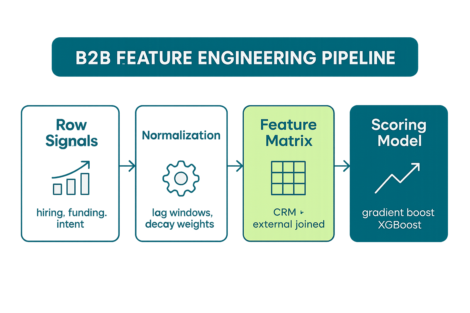
Entity resolution is the first and most critical step. External data sources key on different identifiers: some use domain, some use LinkedIn URL, some use DUNS number, some use a proprietary company ID. Your CRM likely uses Salesforce Account ID or HubSpot Company ID. Before any features can be computed, you need a reliable mapping from your internal account identifier to the external data source identifiers. Explorium’s matching engine handles this with 97.8%+ accuracy across 150 million company profiles, but if you are building this yourself, plan for a probabilistic matching layer that combines domain, company name normalization, and geographic attributes.

Once entity resolution is stable, the pipeline splits into parallel enrichment tracks for each signal category. Each track has different latency requirements. Firmographic enrichment can be batched daily or weekly. Intent signals should be refreshed weekly at minimum. Behavioral signals may need to be near-real-time. Design each track independently and join them at the feature store layer, not the ingestion layer.

import pandas as pd
import numpy as np
from sklearn.preprocessing import StandardScaler, LabelEncoder
from sklearn.impute import KNNImputer
from datetime import datetime, timedelta

# -------------------------------------------------------
# B2B Lead Scoring: External Signal Feature Engineering
# -------------------------------------------------------

def build_firmographic_features(df: pd.DataFrame) -> pd.DataFrame:
    """
    Transform raw firmographic enrichment into model-ready features.
    Assumes df has columns: employee_count, revenue_usd, founded_year,
    industry_code, funding_total_usd, funding_rounds, is_public
    """
    features = df.copy()

    # Log-transform skewed financial fields
    for col in ['employee_count', 'revenue_usd', 'funding_total_usd']:
        features[f'{col}_log'] = np.log1p(features[col].clip(lower=0))

    # Company age as of scoring date
    current_year = datetime.now().year
    features['company_age_years'] = current_year - features['founded_year'].fillna(current_year - 5)

    # Revenue per employee as efficiency proxy
    features['revenue_per_employee'] = (
        features['revenue_usd'] / features['employee_count'].clip(lower=1)
    ).clip(upper=1e7)
    features['revenue_per_employee_log'] = np.log1p(features['revenue_per_employee'])

    # Funding velocity: total funding / company age
    features['funding_velocity'] = (
        features['funding_total_usd'].fillna(0) /
        features['company_age_years'].clip(lower=1)
    )

    # Growth stage encoding (ordinal)
    stage_map = {
        'seed': 1, 'series_a': 2, 'series_b': 3,
        'series_c': 4, 'growth': 5, 'public': 6, 'unknown': 0
    }
    features['funding_stage_ordinal'] = (
        features['funding_stage'].str.lower()
        .map(stage_map)
        .fillna(0)
        .astype(int)
    )

    return features


def build_intent_features(intent_df: pd.DataFrame,
                           topic_weights: dict,
                           windows: list = [7, 14, 30]) -> pd.DataFrame:
    """
    Transform weekly Bombora intent topic scores into time-windowed features.
    intent_df: rows are (company_id, week_end_date, topic, score)
    topic_weights: dict mapping topic -> ICP relevance weight
    windows: list of day windows for rolling aggregation
    """
    intent_df = intent_df.copy()
    intent_df['week_end_date'] = pd.to_datetime(intent_df['week_end_date'])

    # Weight raw intent score by topic relevance to ICP
    intent_df['weighted_score'] = (
        intent_df['score'] *
        intent_df['topic'].map(topic_weights).fillna(0.1)
    )

    today = pd.Timestamp.now().normalize()
    feature_rows = []

    for company_id, group in intent_df.groupby('company_id'):
        row = {'company_id': company_id}
        for window in windows:
            cutoff = today - timedelta(days=window)
            recent = group[group['week_end_date'] >= cutoff]
            row[f'intent_score_sum_{window}d'] = recent['weighted_score'].sum()
            row[f'intent_topic_count_{window}d'] = recent['topic'].nunique()
            row[f'intent_max_score_{window}d'] = recent['weighted_score'].max() if len(recent) > 0 else 0
        feature_rows.append(row)

    return pd.DataFrame(feature_rows)


def apply_waterfall_imputation(df: pd.DataFrame,
                                priority_cols: dict) -> pd.DataFrame:
    """
    Waterfall imputation: fill missing values by cascading across
    equivalent columns from different data sources.
    priority_cols: dict mapping canonical field -> ordered list of source columns
    Example: {'employee_count': ['emp_count_src1', 'emp_count_src2', 'emp_count_src3']}
    """
    result = df.copy()
    for canonical, sources in priority_cols.items():
        result[canonical] = np.nan
        for source in sources:
            if source in result.columns:
                result[canonical] = result[canonical].combine_first(result[source])
    return result

The code above illustrates three of the most important feature engineering primitives for B2B lead scoring. The firmographic feature builder handles the log transformations and derived ratios that prevent skewed distributions from dominating gradient-based models. The intent feature builder implements time-windowed aggregation with ICP-weighted scoring — a pattern that consistently outperforms simple sum aggregation in our evaluations. The waterfall imputation function implements the cascading fill logic that is central to managing feature coverage across multiple data sources.

For a detailed treatment of how waterfall enrichment works across data providers, see our article on waterfall enrichment for B2B data. The key insight is that no single data provider has complete coverage of any attribute, but the union of 3 to 5 providers typically achieves 85 to 95% coverage on core firmographic fields.

Dealing with Sparse and Missing Signals at Scale

Missing data is not a failure of your pipeline. It is a structural property of B2B external signals, and how you handle it has a larger impact on model performance than almost any other engineering decision. The naive approach — dropping rows with missing values or filling with global means — destroys information and introduces systematic bias. Accounts with missing enrichment data are not a random sample. They are systematically skewed toward smaller companies, newer companies, or companies that maintain minimal digital footprint. If you fill their employee count with the global mean, you are lying to your model about who these accounts are.

The right approach depends on the signal type and the downstream model. For tree-based models (XGBoost, LightGBM), you can often pass NaN directly and let the model learn the optimal split for missing values natively. This is the simplest and often best approach for firmographic fields. For neural networks and linear models, you need explicit imputation, and the choice of imputation strategy matters significantly.

The missingness indicator pattern deserves special attention. When a signal is missing for a structurally meaningful reason (a company has no funding data because it is bootstrapped, or has no intent signal because it is too small to appear in B2B research panels), the missingness itself is a feature. Adding a binary column is_revenue_missing alongside a filled revenue column allows the model to learn different behavior for the two populations independently. This typically improves AUC by 1 to 3 points on datasets with high missingness rates.

Coverage improvement through waterfall enrichment is the other lever. Rather than accepting whatever a single provider returns, cascade through multiple providers in priority order. If your primary firmographic provider returns null for employee count, immediately query a secondary provider. Explorium’s enrichment infrastructure does this natively across 50+ data sources, which is why coverage rates for enriched pipelines are typically 85 to 95% compared to 60 to 75% for single-source pipelines. This is not just a data quality improvement — it directly reduces the number of accounts your model has to score with degraded feature vectors, which improves both precision and recall at the top of the funnel.

For deep dives into managing multi-source B2B data enrichment, see our guide on B2B data enrichment and our technical overview of B2B data APIs for lead scoring.

Understanding and Combating Model Drift in B2B Scoring

Model drift in B2B lead scoring is underdiagnosed. Most teams notice it when sales starts complaining that the scores feel wrong, by which point the model has been operating in a degraded state for weeks or months. The challenge is that B2B drift is multidimensional: it can come from label distribution shifts, feature distribution shifts, or the breakdown of the relationship between features and labels. External signals make all three dimensions worse.

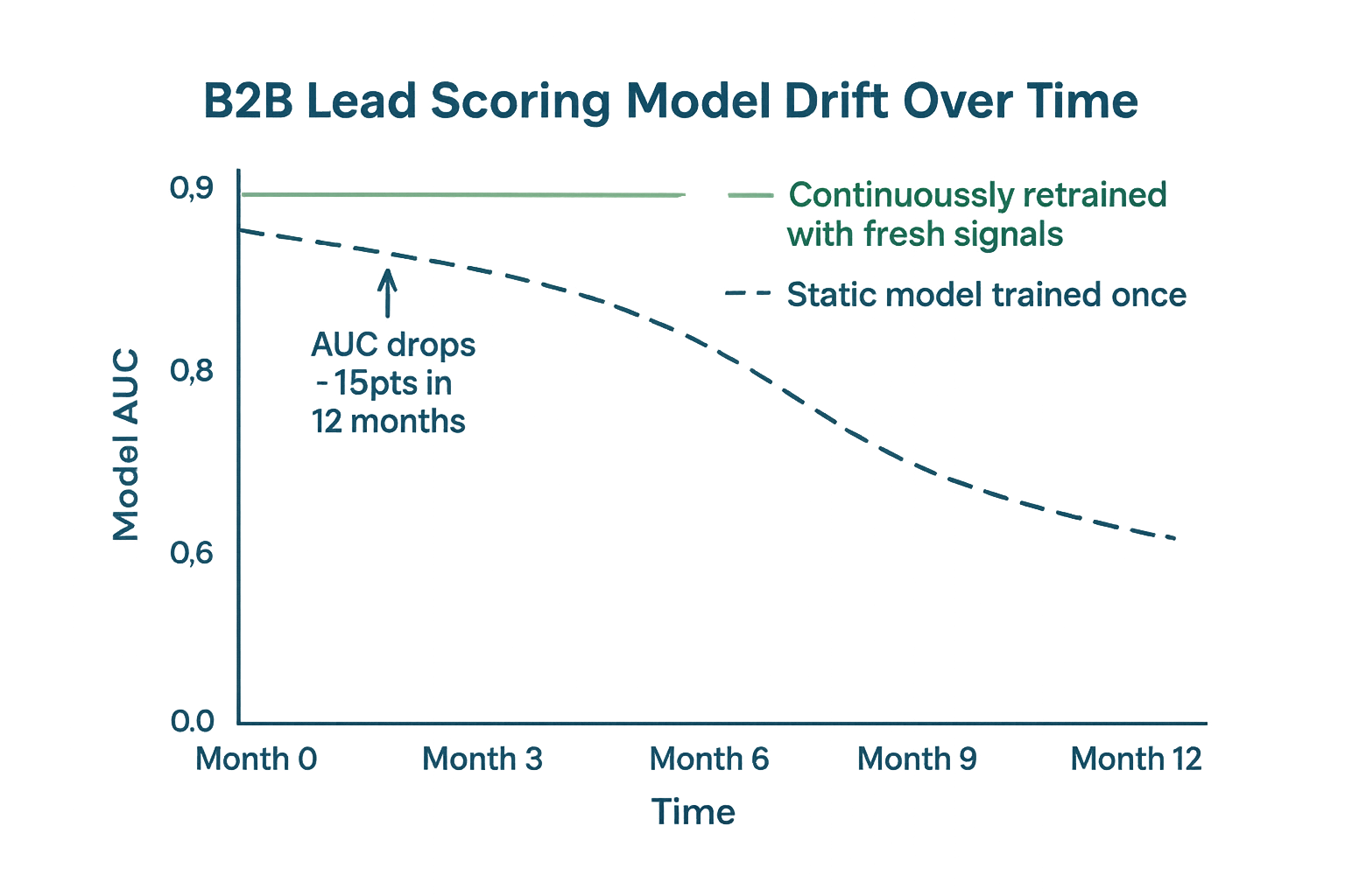
Label drift is the most commonly discussed. If your model was trained during a period of high market velocity and the market slows, the base rate of conversion drops and your model is calibrated incorrectly — not because the features are wrong, but because the prior has shifted. The fix is straightforward: retrain periodically and use isotonic regression or Platt scaling to recalibrate predicted probabilities without full retraining.

Feature drift is more insidious and more common when external signals are in the feature set. Consider what happens to intent signal distributions during macroeconomic contractions. Research activity on enterprise software categories drops broadly. Your model was trained in a period where high intent scores were a strong positive signal. Now high intent scores are rarer and may indicate different things. The relationship between intent score magnitude and conversion probability has shifted, but your model coefficients have not. This is covariate shift, and it cannot be fixed by recalibration alone — it requires retraining on recent data.

Technographic drift is slower but equally real. If a major platform in your ecosystem (say, a cloud provider or CRM) has a rapid adoption surge in your target market, the base rate of companies showing that technographic signal shifts dramatically. Features that were discriminative when 20% of your ICP ran that technology become less discriminative when 70% do. Monitoring feature distributions over time using population stability index (PSI) is the standard technique for detecting this.

import numpy as np
import pandas as pd
from scipy import stats

# -------------------------------------------------------
# Model Drift Detection for B2B Lead Scoring Pipelines
# -------------------------------------------------------

def compute_psi(expected: np.ndarray,
                actual: np.ndarray,
                bins: int = 10) -> float:
    """
    Population Stability Index (PSI) for detecting feature drift.
    PSI < 0.1: No significant change
    PSI 0.1-0.2: Moderate change, monitor closely
    PSI > 0.2: Significant drift, consider retraining
    """
    # Build bins from expected (training) distribution
    breakpoints = np.nanpercentile(expected, np.linspace(0, 100, bins + 1))
    breakpoints = np.unique(breakpoints)  # Handle duplicates

    expected_counts = np.histogram(expected, bins=breakpoints)[0]
    actual_counts = np.histogram(actual, bins=breakpoints)[0]

    # Avoid division by zero
    expected_pct = np.where(expected_counts == 0, 0.001, expected_counts / len(expected))
    actual_pct = np.where(actual_counts == 0, 0.001, actual_counts / len(actual))

    psi = np.sum((actual_pct - expected_pct) * np.log(actual_pct / expected_pct))
    return float(psi)


def monitor_feature_drift(train_df: pd.DataFrame,
                           production_df: pd.DataFrame,
                           feature_cols: list,
                           threshold: float = 0.2) -> pd.DataFrame:
    """
    Compute PSI for all features and flag those exceeding threshold.
    Returns a summary DataFrame sorted by drift severity.
    """
    results = []
    for col in feature_cols:
        if col not in train_df.columns or col not in production_df.columns:
            continue
        train_vals = train_df[col].dropna().values
        prod_vals = production_df[col].dropna().values
        if len(train_vals) < 30 or len(prod_vals) < 30:
            continue
        psi_score = compute_psi(train_vals, prod_vals)
        results.append({
            'feature': col,
            'psi': round(psi_score, 4),
            'drift_severity': (
                'critical' if psi_score > 0.25
                else 'moderate' if psi_score > 0.1
                else 'stable'
            ),
            'retrain_recommended': psi_score > 0.2
        })

    return (pd.DataFrame(results)
              .sort_values('psi', ascending=False)
              .reset_index(drop=True))


def score_label_drift(train_labels: pd.Series,
                      recent_labels: pd.Series,
                      window_days: int = 90) -> dict:
    """
    Test for label distribution shift using chi-square test.
    """
    train_rate = train_labels.mean()
    recent_rate = recent_labels.mean()
    _, p_value = stats.chisquare(
        [recent_labels.sum(), len(recent_labels) - recent_labels.sum()],
        f_exp=[train_rate * len(recent_labels),
               (1 - train_rate) * len(recent_labels)]
    )
    return {
        'train_conversion_rate': round(train_rate, 4),
        'recent_conversion_rate': round(recent_rate, 4),
        'rate_change_pct': round((recent_rate - train_rate) / train_rate * 100, 2),
        'p_value': round(p_value, 4),
        'label_drift_detected': p_value < 0.05
    }

Running PSI monitoring weekly on your external signal features gives you an early warning system that is far more sensitive than waiting for business metrics to degrade. Set up automated alerts when any feature exceeds PSI 0.2, and have a lightweight retraining pipeline ready to trigger. The most sophisticated teams run shadow scoring — evaluating a newly retrained model alongside the production model on real traffic — before cutting over, which minimizes the risk of deploying a model that overfit to recent noise.

For B2B teams specifically, the buying signals category is particularly volatile. See our article on B2B buying signals for a framework on which signal types tend to be most stable versus most volatile across market cycles.

Ready to enrich your lead scoring pipeline? Explorium gives data scientists access to 150M+ company profiles and 800M+ people profiles via API. See how it works →

Measuring Feature Importance with SHAP Values and Permutation Importance

Feature importance in B2B lead scoring is not just a model explainability exercise. It is a business decision framework. Every external signal you include in your feature set has a cost — data licensing fees, API call costs, engineering maintenance overhead, latency added to the scoring pipeline. When you can quantify how much each signal category contributes to model performance, you can make principled decisions about which data investments to expand and which to cut.

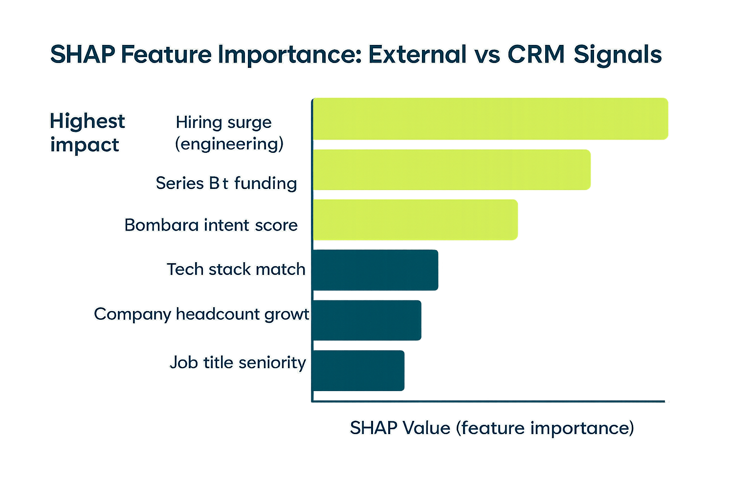
The two most reliable techniques for production feature importance in B2B scoring are SHAP (SHapley Additive exPlanations) values and permutation importance. They measure different things and are complementary. SHAP values decompose each individual prediction into the marginal contribution of each feature, and they respect feature interactions. Permutation importance measures the drop in model performance when a feature's values are randomly shuffled, which captures both main effects and interaction effects. For external signal evaluation, we recommend running both and treating discrepancies as a signal worth investigating.

In practice, the features that consistently show up in the top 20% of SHAP importance for B2B lead scoring pipelines include: intent score in the 7 to 14 day window (the shortest window that captures active research without noise from completed evaluations), technographic fit score (a composite of how closely the account's tech stack matches your best customers), employee count growth rate over 6 months (companies adding headcount are often in expansion mode), and recent funding events within 90 days. These four features alone account for 40 to 60% of total model lift in most B2B scoring applications we have analyzed.

One nuance worth highlighting: static industry codes consistently show low permutation importance in enriched models, but they are still necessary because they anchor the model's base rate calibration. If you drop them, you will often see a small decrease in overall AUC but a larger decrease in calibration quality within specific verticals. Keep table-stakes features even if their individual SHAP scores are low — they provide structural grounding that higher-signal features cannot replace.

The leadership change event row illustrates another pattern: high engineering cost, relatively low average importance, but a high ceiling for specific ICP segments. In accounts where your buyer persona is typically a VP or C-level hire, leadership change events within 30 days are among the most predictive signals available. The average importance looks modest because leadership changes are sparse (10 to 30% coverage), but conditional on the event firing, the lift is enormous. This is a case where segment-specific feature importance analysis yields different conclusions than population-level analysis. For more context on how AI-powered lead generation frameworks handle these conditional signal patterns, see our article on AI lead generation.

How Explorium Solves the External Signal Integration Problem

The engineering challenges described in this article — entity resolution, waterfall enrichment, temporal feature construction, drift monitoring, and real-time scoring — are individually solvable but collectively represent months of infrastructure work before a single model can be trained. Most data science teams building B2B lead scoring in-house spend more time plumbing data than engineering features or evaluating models. Explorium was built to collapse that infrastructure work into an API call.

At the data layer, Explorium aggregates 150 million company profiles and 800 million people profiles across 50+ data sources, applying the entity resolution and waterfall enrichment logic described above before any data reaches your pipeline. The 97.8%+ company match accuracy means that when you query by domain or company name, you are getting the right account's signals, not a false match. The 18 signal categories and 80+ buying signal types cover the full taxonomy described in this article: firmographic, technographic, intent (including Bombora intent topics), behavioral, and news/event signals are all available through a unified API surface.

For data scientists who need to integrate external signals into training pipelines and production scoring workflows, the AgentSource MCP server is the practical interface. It supports 100 QPS synchronous requests, which is sufficient for real-time scoring on inbound lead flows (most inbound lead flows are 1 to 10 leads per second at peak, well within the synchronous limit) and for batch enrichment of full CRM exports (a 100,000-account CRM export at 100 QPS takes roughly 17 minutes). The API returns structured JSON feature vectors that are designed to drop directly into pandas DataFrames or feature store schemas, minimizing transformation overhead.

For teams that want to evaluate which signal categories are worth licensing before committing to full pipeline integration, Explorium supports targeted signal queries: you can pull only intent signals for a cohort, or only technographic data for a list of domains, which lets you run offline A/B tests of feature value before changing production infrastructure. This is the methodology we recommend: pull a historical cohort of won and lost opportunities, enrich them retroactively with external signals, train a model, and compare holdout AUC to your current production model. The delta tells you exactly what the enrichment is worth in model performance terms before you invest in production integration.

See our overview of B2B data enrichment approaches for context on how to structure that evaluation, and our guide to B2B data APIs for lead scoring for the technical integration patterns most commonly used by our data science customers.

Real-World Signal Impact: Case Studies and Benchmark Evidence

Abstract arguments about signal value are useful, but practitioners need to see actual numbers. The following section documents signal impact patterns observed across B2B lead scoring use cases, drawing on consistent patterns in what works and what does not across different company sizes, verticals, and sales motions.

In a mid-market SaaS use case selling to companies with 100 to 1,000 employees in the technology sector, adding a 14-day intent score composite (weighted across 12 Bombora topics mapped to the product category) to a baseline model that included firmographic and CRM activity features improved AUC from 0.74 to 0.81. That 7-point improvement translated into a 34% improvement in sales-accepted opportunity rate in the top scoring decile, meaning the sales team was spending less time on accounts that did not convert and more time on accounts that did. The key engineering decision that produced this result was the 14-day window (not 30, not 7): the 14-day window captured companies in active evaluation while excluding research activity from completed purchase cycles.

In an enterprise SaaS use case selling to companies with 1,000+ employees, the most impactful single feature was not intent but technographic fit: specifically, a composite score that measured the overlap between the target account's observed tech stack and the tech stack profile of the top quartile of existing customers. This feature had lower AUC lift than intent (about 4 points versus 7) but was far more stable across time and required no high-frequency data refresh. For enterprise deals with 6 to 18 month cycles, technographic fit turned out to be a better leading indicator than short-window intent because enterprise research cycles are longer and noisier.

For a financial services data provider targeting compliance-adjacent buyers, news and event signals were the surprise winner. Leadership change events (specifically, new Chief Compliance Officers or Chief Risk Officers joining target accounts within the past 60 days) produced an 11x lift in conversion rate relative to accounts with no leadership change event. The coverage was low (about 18% of accounts had a detectable leadership change in any 60-day window) but the signal was so strong that it justified building a dedicated model pathway for the high-signal cohort versus a general model for the rest. This is the segmented modeling approach: rather than one model for all accounts, use signal availability to segment and train specialized models with appropriate features for each segment.

For teams building or evaluating their first external signal pipeline, our guide to B2B buying signals covers the prioritization framework in more depth, and our article on AI-powered lead generation covers how these scoring systems feed into automated GTM workflows.

FAQs

What is the most important external signal to add first to a B2B lead scoring model?

If you are starting from a CRM-only baseline, the highest-ROI first addition is typically a short-window intent signal (7 to 14 days) weighted by topic relevance to your ICP. Intent data consistently produces the largest single AUC improvement because it captures active in-market behavior rather than static attributes. Bombora intent topics are the industry standard for B2B intent data coverage. The engineering requirement is manageable — weekly API calls per account in your CRM — and the signal requires no entity resolution beyond domain matching. Most teams see a 5 to 8 point AUC improvement from this single addition, which is enough to justify the data licensing cost within the first quarter of deployment.

How do you handle companies that do not appear in external data sources?

Missing enrichment coverage is highest for very small companies (under 20 employees), very new companies (under 2 years old), and companies in emerging markets with lower digital footprint. The recommended approach is threefold. First, use waterfall enrichment across multiple providers to maximize coverage before declaring a record unenrichable. Second, build a separate lightweight model for unenrichable accounts that uses only first-party signals (website behavior, email engagement, self-reported form data). Third, add a binary feature indicating enrichment availability to the main model so it can learn that unenrichable accounts have different base conversion rates. Do not drop unenrichable accounts from scoring entirely — they still convert, just at different rates.

How often should a B2B lead scoring model be retrained when external signals are in the feature set?

External signals accelerate the need for retraining compared to CRM-only models. A practical cadence for most B2B teams is monthly retraining for intent-heavy models and quarterly retraining for firmographic-heavy models, with trigger-based retraining when PSI exceeds 0.2 on any top-10 feature. The key infrastructure requirement is automating the training pipeline so retraining is cheap. If retraining requires manual intervention, teams delay it and accumulate drift. Invest in automated retraining infrastructure before you invest in more signal categories. A well-tuned model on existing signals will outperform a poorly maintained model with richer signals every time.

What is the difference between permutation importance and SHAP values for feature selection in B2B scoring?

Permutation importance measures the drop in overall model performance when a feature is randomly shuffled, capturing both main effects and interaction effects in aggregate. It answers the question: how much does this feature contribute to the model’s overall discriminative power? SHAP values decompose individual predictions into feature contributions, respecting feature interactions and providing instance-level explanations. For feature selection decisions, permutation importance is faster and gives you a cleaner signal about which features to drop. For understanding why specific accounts are scored the way they are — which is important for sales enablement and model auditing — SHAP values are more useful. Use permutation importance for feature pruning and SHAP values for explainability and investment prioritization.

Can external signal features cause regulatory or compliance issues in lead scoring?

Yes, and this is an underappreciated risk in B2B ML pipelines. Using individual-level behavioral data (personal browsing behavior, individual email engagement at named contacts) in scoring models may trigger GDPR, CCPA, or sector-specific compliance requirements depending on your market and buyer geography. Company-level signals — firmographic data, company-level intent scores, technographic attributes — are generally lower risk because they describe the organization rather than named individuals. When in doubt, consult legal counsel and design your feature engineering pipeline to use company-level aggregates rather than individual-level signals. Explorium’s data products are designed with this boundary in mind, providing company-level aggregates that preserve predictive power while reducing individual data exposure.